ASR with Weighted Finite State Transducers
In this post, the subject of decoders for Automatic Speech Recognition was introduced, presenting the task of searching for the best word sequence given an audio observation. One solution for that involves the use of Weighted Finite State Transducers (WFSTs). This post is theory heavy, so don’t worry if you don’t understand all of it on first try (I certainly didn’t).
WFSTs are static graphs encoding the whole word-sequence search space. They contain many levels of information, going from the acoustic model to phones in context, to single phonemes, to words, and finally, words in sequence.
A finite-state transducer is a finite automaton whose state transitions are labeled with both input and output symbols. Therefore, a path through the transducer encodes a mapping from an input to an output string. They provide a common and natural representation for major components of speech recognition systems, including Hidden Markov Models (HMMs), context-dependency models, pronunciation dictionaries, statistical grammars and word or phone lattices [1]. The decoder goes through the WFST creating a lattice, a graph structure that contains the most probable - or less costly - paths for a given utterance (a continuous piece of speech beginning and ending with a clear pause), taking into account both acoustic and language costs.
A transducer $T=(\mathcal{A}, \mathcal{B}, \mathcal{Q}, I, F, E, \lambda, \rho)$ over a semiring $\mathbb{K}$ is characterized by:
- $\mathcal{A}$: finite input alphabet;
- $\mathcal{B}$: finite output alphabet;
- $\mathcal{Q}$: finite set of states;
- $I$: set of initial states;
- $F$: set of final states;
- $E$: finite set of transitions;
- $\lambda$: initial state weight assignment;
- $\rho$: final state weight assignment.
The set of transitions is $E\subseteq\bar{E}=\mathcal{Q}\times(\mathcal{A}\cup{\epsilon})\times(\mathcal{B}\cup{\epsilon})\times\mathbb{K}\times\mathcal{Q}$. This means it is a subset of all possibilities of transition from one state to another (or to itself) with an input label, an output label and a weight. $\epsilon$ means an empty label, no input or no output.
The operations are executed on specific semirings. A semiring is a set $\mathbb{R}$ equipped with two binary operators addition ($\oplus$) and multiplication ($\otimes$), with identity elements $\bar{0}$ and $\bar{1}$, respectively. One simple example of a semiring is the set of natural numbers (including zero) under ordinary addition and multiplication [2]. Two commonly used semirings in ASR are the probability semiring and the log semiring, shown in Table 1.
| SEMIRING | SET | $\oplus$ | $\otimes$ | $\bar{0}$ | $\bar{1}$ |
|---|---|---|---|---|---|
| Probability | $\mathbb{R}_+$ | $+$ | $\times$ | 0 | 1 |
| Log | $\mathbb{R} \cup {-\infty,+\infty}$ | $\oplus_{log}$ | + | $+\infty$ | 0 |
Table 1: Probability and log semirings. $\oplus_{log}$ is defined by: $x \oplus y=-log(e^{-x}+e^{-y})$.}
There is a set of operations we can perform on transducers. The main ones are the following:
- Composition: Combining graphs, therefore different levels of representation;
- Determinization: Making an automaton deterministic, that is, each state should have at most one transition with any given input label, which should not be the empty ($\epsilon$) symbols;
- Minimization: Reducing the size of a deterministic automaton.
A widely used toolkit for ASR is Kaldi [3]. A usual decoder in Kaldi contains a set of four WFSTs which are combined (or composed, as explained below): HMM-level, Context Dependency, Pronunciation Lexicon and Grammar. The mapping from input to output across transducers is shown in Figure 1.
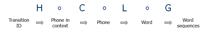
Figure 1: Mapping of input and output across transducers.
Figure 2 is the representation of a grammar with full sentences. Arcs show legal word strings and their probabilities. As input and output labels are the same, we call this automaton an acceptor (it ends at a final state if the sequence is accepted by the WFST). The graph in Figure 3 corresponds to a pronunciation lexicon, showing different possibilities of pronunciation and mapping a phone string to a word string in the lexicon. Since it transduces phones to words, it is called a transducer. Here are some Weighted finite-state transducer examples:
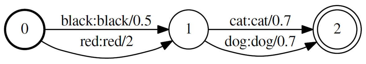
Figure 2: Example grammar FST.
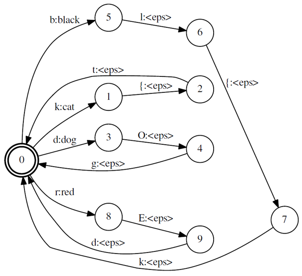
Figure 3: Example pronunciation lexicon FST.
Essentially, the grammar graph shows us the allowed sequences of words along with the probability of their occurrence. It can be hand crafted through the use of regular expressions, rules or even direct build, but it can most notably be learned from data, creating stochastic $n$-gram models from text corpora.
The lexicon graph, on the other hand, presents the allowed pronunciations for the words. It is the Kleene closure of the union of individual word pronunciations, that is, the set of pronunciations for all word sequences. This means that there are loops in this automaton. For matters of efficiency, output word labels should be placed on the initial transition of words.
Below is a visual example of graph growth with composition of H, C, L and G transducers.
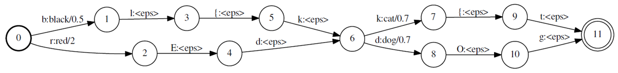
Figure 4: Example $L\circ G$.
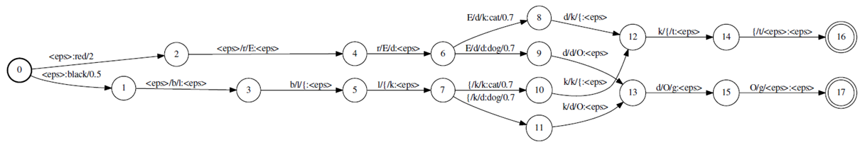
Figure 5: Example $C\circ L\circ G$.
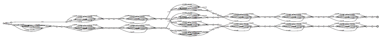
Figure 6: Example $C\circ L\circ G$.
The operation of composition essentially consists in checking transitions in both input transducers and adding an arc to the output graph whenever the output label of the first transducer matches the input of the second one. This creates a mapping between the input of $T_1$ and the output of $T_2$. A visual example, also from [2], is shown in Figure 7. It works like function composition, where the composition $(f\circ g)(x)$ of function $f$ with function $g$ is equal to $f(g(x))$.
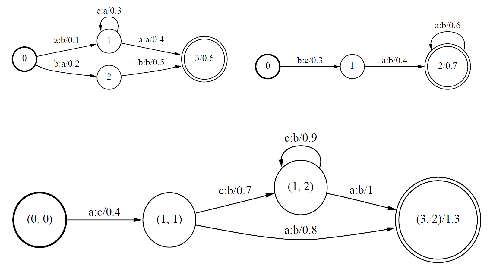
Figure 7: Example of a basic transducer composition [1]. The upper left transducer is $T_1$, the upper right one is $T_2$, and the graph below them is the result.
During decoding, the decoder examines the word-sequence search space beginning with start states and evaluates transition costs in order to build a lattice, a representation of the alternative $n$-best word-sequences
Below is an illustration of decoding operation. For each time frame, visited states are saved in the form of tokens, with links to other states. Notice how not all states and transitions make their way into the lattice (and those that are there can still be removed via pruning).
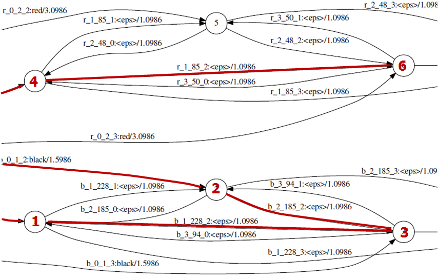
Figure 8: Example FST examined during decoding.
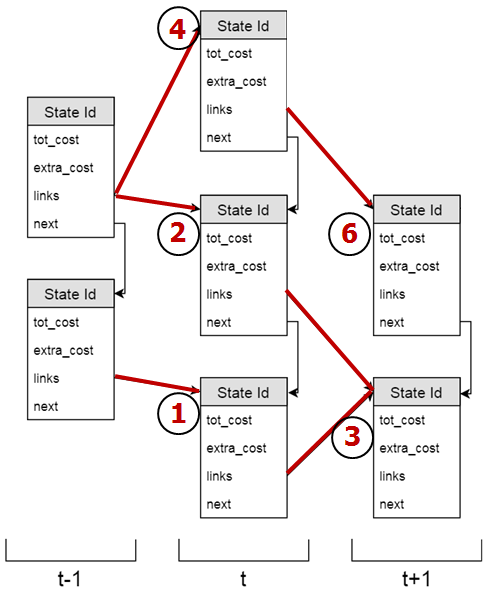
Figure 9: Example lattice created from decoding.
Kaldi creates a data structure corresponding to a full state-level lattice, so for every arc of $HCLG$ traversed, a separate arc is created in the lattice, with acoustic and graph cost stored separately, as illustrated in Figure 9. This structure is pruned periodically, and the final pruned graph then has its epsilons removed and is determinized [4].
More on the theory of weighted finite state transducers can be found in [1]. For more on Kaldi, check out their documentation page.
Comments